Stopwatches, pendulums and bell curves
A simple experiment to show what random error is, how it affects uncertainty in a measurement and how it can be managed with statistics
Whenever we take a measurement, we introduce an error associated with it. It’s one of life’s hard truths, and one that will laugh you in the face if you ever try to buy a bookcase roughly the same size as an alcove in your wall.
The thing is, when the mason told you that space was going to be 1 m wide, and the IKEA product sheet told you the width of the furniture would be 99 cm, they were both right in their own way. Still, your bookcase might not fit.
What happened? Well, they just have different uncertainties in their measurements.
What is uncertainty?
If you have ever looked at a technical sheet, you might have seen that physical values often come with a ± sign. For example, the accuracy of a temperature sensor might be reported as ± 0.2 °C.
The manufacturer is telling you that the true value of the measured quantity is expected to sit inside that range under some stated conditions. Sometimes that range is a maximum error bound, sometimes it is a statistical confidence interval, and sometimes you need to read the fine print to know which one.
Going back to our bookcase, it’s easy to see what went wrong. The mason’s job introduces more chances for error. When he tells you the space is 1 meter wide, he may implicitly mean something like 100 cm ± 1 cm, while the IKEA product sheet, due to a much more controlled and standardized manufacturing process, may mean 99 cm ± 0.2 cm. Those two intervals overlap. The opening could be a little smaller than planned, the bookcase could be a little larger than advertised, and suddenly the comfortable-looking 1 cm margin disappears.
Managing uncertainty with statistics
It might seem that your ability to make a measurement is limited by the resolution of your instruments, but that’s not the whole story: you have to account for the whole measurement process. If you’re trying to time something with a stopwatch, even if it has a resolution of 0.001 s, you might be off by 0.1 s or more simply because you’re human and you might be too early or too late when pressing the lap button.
Thankfully, we have a way to deal with this kind of random error: repaeated sampling!
The concept is intuitive enough; it’s why your nutritionist might tell you to weigh yourself more than once during the day and take an average: your weight can have some random fluctuations, and averaging makes part of that noise cancel out, assuming those fluctuations are not all biased in the same direction.
The following experiment has you timing the swing of a pendulum multiple times and takes care of computing and interpreting the underlying statistics for you.
Note that you could do it yourself with a good pendulum, a stopwatch and a spreadsheet, and I encourage you to do so if you have the time.
What the experiment is measuring
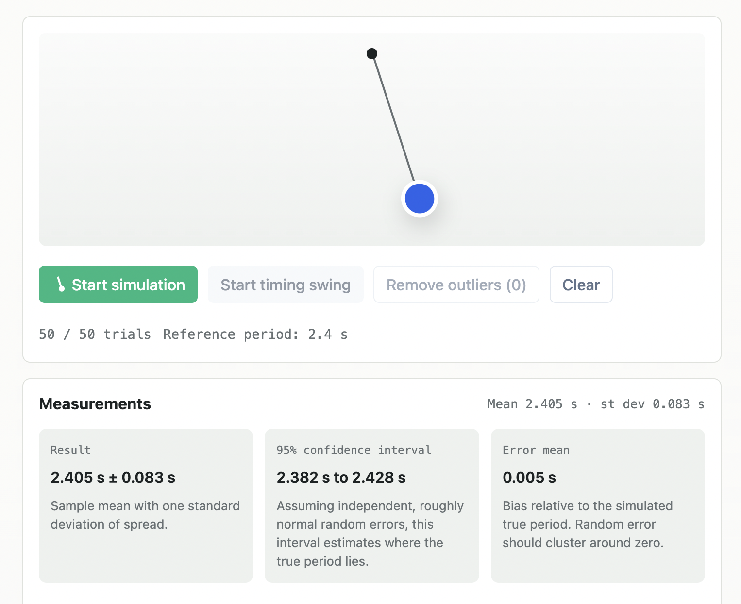
Spoiler: the simulated pendulum has a true period of 2.4 s. In a real experiment, this is the value we would be trying to estimate, maybe to test if the pendulum’s equation of motion holds. Here it is known by the program, which lets the demo show the error of each attempt.
What you should take away is that the more measurements you take (the demo lets you go up to 50), that is, the bigger your sample size is, the more the mean should converge towards the expected value, which makes your 95% confidence interval tighten and the mean error converge to 0.
If you make an obvious mistake (such as recording an half swing or forgetting to stop the recording), you can just keep going and then press the “remove outliers” button when your previous error is identified as an outlier.
An in depth explanation of how it all works is available under the experiment.
Measurements
Mean 0.000 s · st dev 0.000 s
Sample mean with one standard deviation of spread.
Assuming independent, roughly normal random errors, this interval estimates where the true period lies.
Bias relative to the simulated true period. Random error should cluster around zero.
| Trial | Measured time | Error |
|---|---|---|
| No measurements yet. | ||
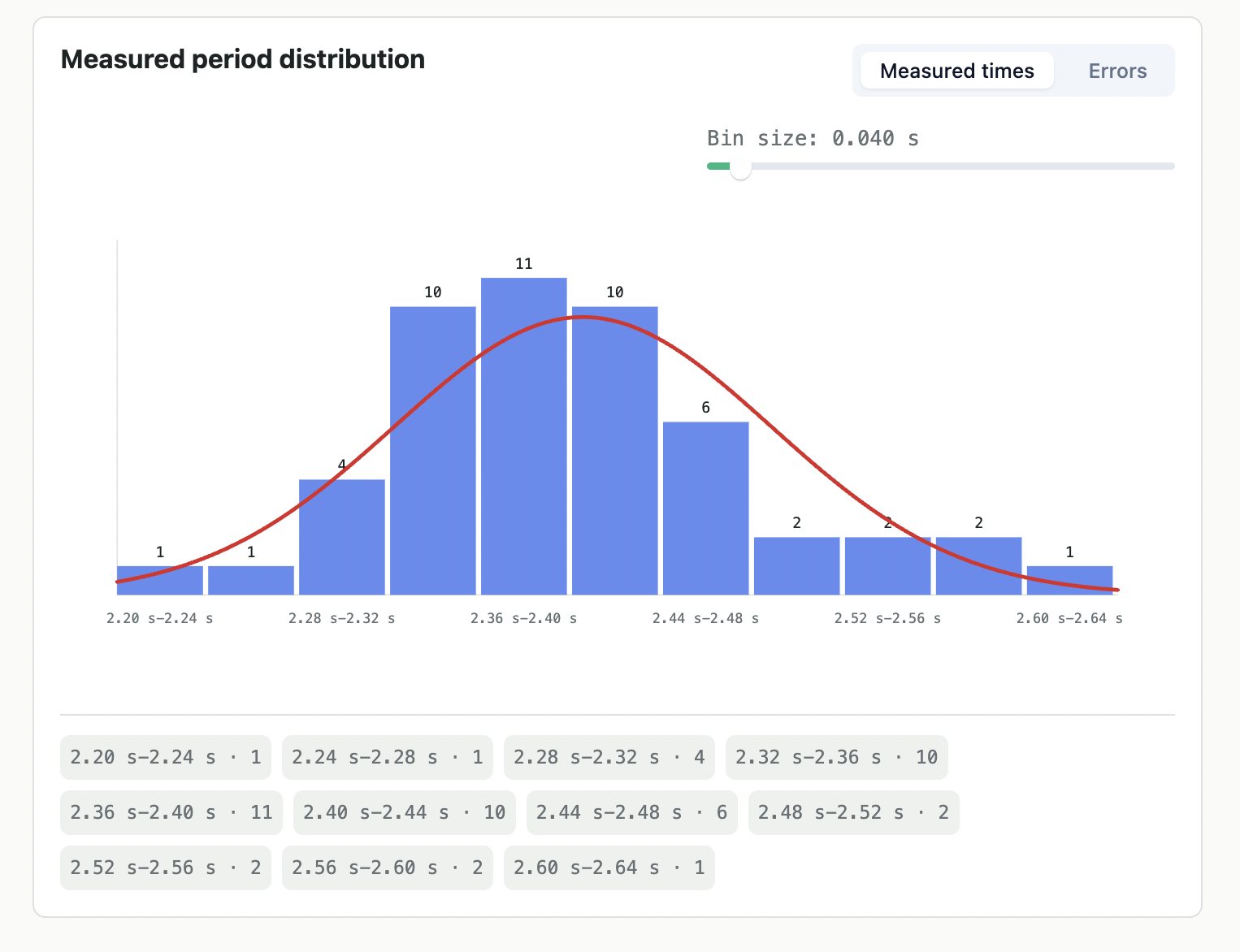
Measured period distribution
In depth
The mean
The sample mean is the average of your measured times:
The mean is our best estimate of the pendulum period. If the timing errors are random and centered around zero, then early and late attempts partially cancel each other out. That is why repeating the measurement helps.
The standard deviation
The sample standard deviation tells us how spread out the individual measurements are around the mean. In this demo it is computed with the sample formula, which divides by .
If you’re curious about why n - 1 is used, you can check out Bessel’s correction.
A small standard deviation means your measurements are tightly clustered. A large standard deviation means your timing process is noisy.
This is the first important distinction:
describes the spread of individual measurements. It does not directly say how uncertain the mean is.
If the errors are approximately normal, about 68% of individual measurements lie within one standard deviation of the mean, about 95% lie within two standard deviations, and about 99.7% lie within three standard deviations. That is the reason the demo has a button to remove measurements more than three standard deviations away from the mean: under a normal-error model, those values are unusual enough to deserve inspection.
Error distribution
The histogram can show either the measured times or the errors. The error view is often more revealing.
If the measurement process is dominated by random timing error, the error histogram should be centered near zero. It may still be rough or slightly skewed, especially with only a few trials, but the general idea is that positive and negative errors both occur.
If the error histogram is clearly shifted away from zero, the experiment has a bias: maybe you tend to stop consistently early or late.
The red curve on the histogram is a Gaussian curve built from the sample mean and sample standard deviation. It is a visual way of saying “if these errors were normal with this mean and this spread, the distribution would look roughly like this.”
Uncertainty of the mean
Now we get to the quantity we usually care about: the uncertainty in the estimated period.
Individual measurements vary with standard deviation , but the mean becomes more stable as the number of measurements increases. The uncertainty of the mean is measured by the standard error:
This is why repeated measurements are powerful. If you take four times as many independent measurements, the uncertainty of the mean is cut in half.
The demo reports a 95% confidence interval for the true period. It uses:
where t is a Student’s t multiplier. For very large samples this multiplier approaches about 1.96, but for small samples it is larger because the standard deviation itself is uncertain.
So when the demo says the true value lies in the 95% confidence interval, the careful interpretation is:
If we repeated this whole experiment many times, and computed a 95% confidence interval each time using the same method, about 95% of those intervals would contain the true period.
It does not mean there is a 95% probability that this one fixed interval contains the true value in a strict frequentist sense. In everyday scientific language people often say it that way informally, but the repeated-experiment interpretation is the precise one.
What validates the result?
Statistics helps validate the result by asking whether the data is consistent with the claim.
For this experiment, a good result should have:
- a mean close to the known period of 2.4 s
- an error mean close to zero
- an error histogram that looks roughly centered, even if imperfect
- a confidence interval that contains 2.4 s
- no unexplained extreme outliers
If all those things are true, then your experiment supports the claimed period of 2.4 s.
Here are the results I got when running the experiment: